
LLM Distillation Explained - Part 1
How It Works and How to Do It

Like most people working in AI these days, I’ve been spending a lot of time with Generative AI and Large Language Models (LLMs). Over the past few months, my focus has been on distributed LLM training across large GPU clusters. Throughout this journey, I’ve been especially intrigued by LLM distillation - a technique that’s both remarkably simple and highly effective at optimizing model training.
Tired of clickbait articles that gloss over the details without offering real explanations or usable code, I’ve decided to write a clear, no-nonsense guide to the process - with practical examples and actual libraries you can use.
In this article, I’ll walk you through the concept of LLM distillation and show you how to implement it in Python. We’ll begin with Logit Distillation techniques and later move on to Hidden State Distillation. The goal of this post is to explain everything straightforwardly, no formulas, just clear intuition. If you’re into equations, you’re welcome to follow along, but this guide focuses more on understanding than math.
Introduction to distillation
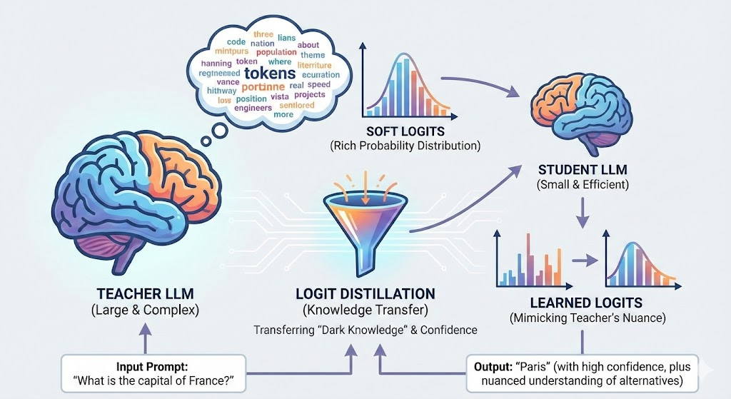
Large Language Models (LLMs) like GPT or LLaMA are powerful but often huge - they require a lot of memory, computation, and energy to run. Distillation is a technique that helps to make these models smaller, faster, and more efficient without losing too much of their intelligence.
Think of it like this: imagine a big, brilliant teacher explaining things to a student. The student doesn’t memorize everything, but learns the essence of how the teacher thinks and responds. Over time, the student becomes good enough to give similar answers, but using fewer resources.
In LLM distillation, the “teacher” is a large pre-trained model, and the “student” is the smaller model we want to train. We let the student learn by imitating the teacher - by observing its responses, predictions, and even how it thinks internally. The result? A much lighter model that can still perform well in real tasks, from chatting to coding - perfect for mobile devices, chatbots, or cost-efficient deployments.
The main idea then is to take a large model like LLama 70B and “distill” its knowledge into a small model like LLama 8B, 4B, or even 1B. This process should also be less computationally expensive compared to “training from scratch” since we use not only the simple “next token” prediction but also the hidden “dark knowledge” [1] of the teacher model. This is the secret sauce of distillation: we extract all the possible information from the model, not only the directly visible one.
Logit distillation? Let’s understand what it is
First, we need to practically understand what dark knowledge is in the context of the Logit distillation. I’ll use the concept of dark knowledge to introduce the logit distillation since they are strongly correlated.
Tokenization
Every time you provide a text input to an LLM, the tokenizer transforms each word or subword into a corresponding integer. Here’s a simple example to illustrate how it works:
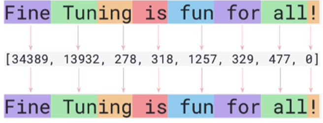
Each token is assigned a unique integer through a dictionary, so every word (or subword) has its own numeric representation. The total number of tokens a tokenizer can handle is called the vocabulary size. This means an LLM can only understand and work with the tokens included in its vocabulary.
For example, Llama3 has a vocabulary size of 128,256, meaning it can process and generate up to 128,256 distinct tokens. Once the text is converted into tokens, the LLM works entirely with their numerical representations - it doesn’t “see” any actual words or text. At the end of the process, it converts these numbers back into text through a step called de-tokenization.
Understanding this concept is crucial to grasping what logit distillation is all about. If any part of this feels unclear, I recommend revisiting it before moving on. And if you’re curious to dive deeper into tokenization, I suggest checking out [2].
Logit generation
Every time you provide input to an LLM, the model calculates a logit value for each token in its vocabulary before converting the output back into text. In simpler terms, with Llama3, this means that at each prediction step, the model produces a vector with 128,256 floating-point numbers - one for every possible token.
Here’s an example to illustrate what that looks like:
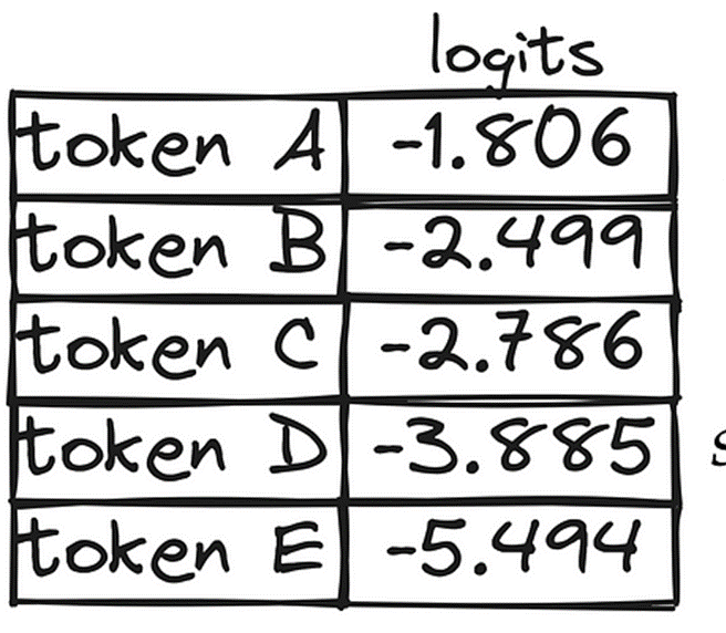
In the context of logit distillation, this table represents the LLM’s “dark knowledge”. Each number corresponds to a logit, which reflects how much importance the model assigns to a specific token. Tokens with higher logit values are more likely to be chosen as the next prediction.
These logits are eventually transformed into probabilities using a softmax function, which also involves a parameter called temperature. But for now, let’s set softmax aside and just focus on understanding what logits are.
Distillation using logits
Now that you are aware of what logits are and how LLMs compute them. We can deep dive into how distillation works. Let’s describe how the algorithm works:
Step 1: Forward pass through both models
For a given input, both the teacher and the student perform the next token prediction, generating an array of logits. Here’s what this looks like in practice:
+--------+---------------------------+---------------------------+
| Token  | Logits (Teacher)          | Logits (Student)          |
+--------+---------------------------+---------------------------+
| “Ceci” | [2.0, 1.0, 4.0, 0.5, 0.3] | [1.9, 1.1, 3.9, 0.6, 0.4] |
| “est”  | [0.5, 3.0, 1.0, 0.2, 0.3] | [0.6, 2.9, 1.1, 0.3, 0.4] |
| “un”   | [0.1, 0.2, 0.5, 4.5, 0.7] | [0.2, 0.1, 0.6, 4.4, 0.8] |
| “test” | [3.5, 1.5, 0.1, 0.0, 0.2] | [3.4, 1.4, 0.2, 0.1, 0.3] |
+--------+---------------------------+---------------------------+
Step 2: Compute the distillation loss
The key insight here is that we want the student’s logit distribution to match the teacher’s logit distribution. This is where the “dark knowledge” comes in - we’re not just teaching the student to predict the correct next token, but to understand the entire probability distribution over all possible tokens that the teacher has learned.
There are two main components to the loss function in logit distillation:
Distillation Loss (Soft Targets): This measures how well the student’s logits match the teacher’s logits. We typically use the KL-divergence (Kullback-Leibler divergence) to measure the difference between the two probability distributions after applying softmax with temperature.
Student Loss (Hard Targets): This is the standard cross-entropy loss between the student’s predictions and the actual ground truth labels from the dataset.
The total loss is a weighted combination of these two:
Total Loss = α × Distillation Loss + (1 - α) × Student LossWhere α is a hyperparameter (typically between 0.5 and 0.9) that controls how much we want the student to learn from the teacher versus the ground truth.
Step 3: The role of temperature
Temperature is a crucial hyperparameter in logit distillation. Before computing the distillation loss, we apply a softmax function with temperature T to both teacher and student logits:
P(token_i) = exp(logit_i / T) / Σ exp(logit_j / T)When T = 1, this is just standard softmax. When T > 1 (typically T = 2 to 5), the probability distribution becomes “softer” - meaning the differences between high and low probability tokens become less extreme. This is important because it reveals more of the teacher’s “dark knowledge” about which tokens are somewhat plausible, even if they’re not the top choice.
Step 4: Backward pass and optimization
Once we have the total loss, we perform a backward pass to compute gradients, but only for the student model. The teacher model remains frozen - we don’t update its weights. The student’s weights are then updated using an optimizer like Adam or SGD.
Why this works
The beauty of logit distillation lies in its efficiency and effectiveness:
The student learns not just what the correct answer is, but also what the teacher considers reasonable alternatives
This richer signal helps the student generalize better than training from scratch
Since both models share the same tokenizer and vocabulary, the logit vectors align perfectly - making the transfer of knowledge seamless
The student can learn from the teacher’s uncertainties and confidence levels, not just from binary correct/incorrect labels
Important note about tokenizer and dictionary
For logit distillation to work in this straightforward way, the teacher and student must share the same tokenizer and vocabulary. Why? Because the logit vectors must have the same dimensionality, and each position must correspond to the same token in both models.
If “hello” is token 1234 in the teacher’s vocabulary, it must also be token 1234 in the student’s vocabulary. Otherwise, we’d be comparing apples to oranges - the teacher’s confidence about token X would be interpreted by the student as confidence about a completely different token Y.
This is why logit distillation is most commonly used within model families like LLaMA 2 → LLaMA 3 or GPT-3 → smaller GPT variants, where the tokenizer remains consistent across different model sizes.
What next
In this first part, we’ve explored the fundamentals of logit distillation - how a large teacher model transfers its “dark knowledge” to a smaller student model through logit matching.
We covered the key concepts: how LLMs generate logit vectors for every token in their vocabulary, why these logits contain richer information than just the predicted token, and how the distillation process works by aligning the student’s logit distribution with the teacher’s using a combination of soft and hard targets with temperature scaling.
We also emphasized an important constraint: this approach requires teacher and student to share the same tokenizer and vocabulary for seamless knowledge transfer.
What’s next? In Part 2, we’ll dive into the practical implementation with Python code, working examples, and the libraries you can actually use to perform logit distillation on your own models.
If you found this article helpful, please subscribe to stay updated when Part 2 drops. We’ll go from theory to practice, giving you everything you need to start distilling your own models.
References
[1] G. Hinton et al. Dark Knowledge 2014, https://www.ttic.edu/dl/dark14.pdf
[2] https://medium.com/illuminations-mirror/on-tokenization-in-llms-34309273f238